Morphospace Visualization Tool

X PC: Y PC:

Source: (--, --)
Target: (--, --)

PC Axes Context

Select different X/Y PCs to see an explanation here.

About the Study

Title: Decoding Shape Diversity: An Autoencoder-Based Morphospace for Comprehensive Biological Shape Analysis

Authors & Affiliations:

Oshane O. Thomas^1*, R. L. Raaum², A. Murat Maga^1,3
1. Center for Development Biology and Regenerative Medicine, Seattle Children’s Research Institute, Seattle, WA
3. Division of Craniofacial Medicine, Department of Pediatrics, University of Washington, Seattle, WA
*Correspondence: oshane.thomas@seattlechildrens.org

Keywords: Functional Map Framework, Geometric Morphometrics, Geometry Processing, Landmarking, Mouse Mandible, Rapid Morphological Phenotyping

Abstract & Goals

This study demonstrates how DISCO-AE can create an interpolatable and interpretable morphospace for comprehensive biological shape analysis. We combine morphVQ-based shape correspondences and an unsupervised autoencoder to facilitate robust morphological phenotyping, bridging the gap between classic landmark-based approaches and dense surface-based methods.

Results Summary

Our experiments show that DISCO-AE produces consistently low reconstruction errors, preserving both broad structural features and subtle morphological details. Principal component axes derived from the learned embeddings capture hierarchical shape variation, from large-scale differences (PC1/PC2) to finer localized contours (PC3+). Quantitative assessments (e.g., partial least squares correlations with size, manifold-quality metrics like residual variance) confirm that the DISCO-AE morphospace is both biologically meaningful and structurally robust, making it an ideal foundation for further comparative analyses.

Key Figures

Click any thumbnail to view a larger version.

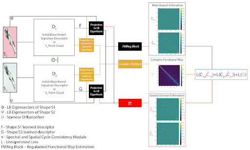
Fig. 1A. morphVQ Network Architecture
Pipeline for obtaining robust shape correspondences

DISCO-AE Architecture
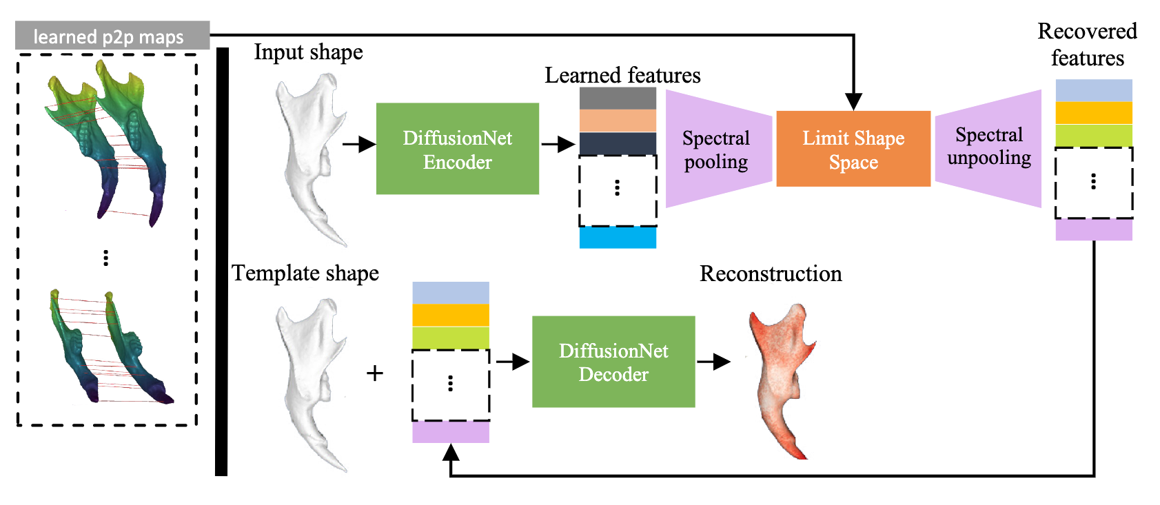
Mesh autoencoder with spectral pooling

Reconstruction Accuracy
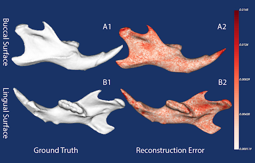
Original vs. reconstructed surfaces + error map

How to Use This Tool

Fetch PCA Data: Click “Fetch PCA Data” to load up to 15 principal components from the server. The chart will display all specimens, color-coded by group.
Select PCs: Use the “X PC” and “Y PC” dropdowns to choose which two principal components to view on the scatter plot. Changing them clears any existing picks or shapes.
Pick Source & Target:
- Click “Set Source” and single-click anywhere in the chart. The chosen point becomes the source (green).
- Click “Set Target” and single-click in the chart for the target (blue).
A dashed gray line indicates the interpolation path between source and target.
Compute & Interpolate: Once both source and target are set, the “Compute & Interpolate” button becomes enabled. Click it to send the points for interpolation to the server.
View 3D Shapes:
- The server returns a series of shapes (aligned) colored by per-vertex error relative to shape #0.
- Use the slider below the scatter plot to step through the shapes [0..N-1].
Repeat:
- You can change the PC axes at any time (this clears shapes and picks), then pick new source/target and run interpolation again.